Classifying metagenomic samples

The classification algorithm

There are three types of results;
1. single-lineage (SL) classifications,
2. split classifications,
3. reads that are not like anything currently in the database.
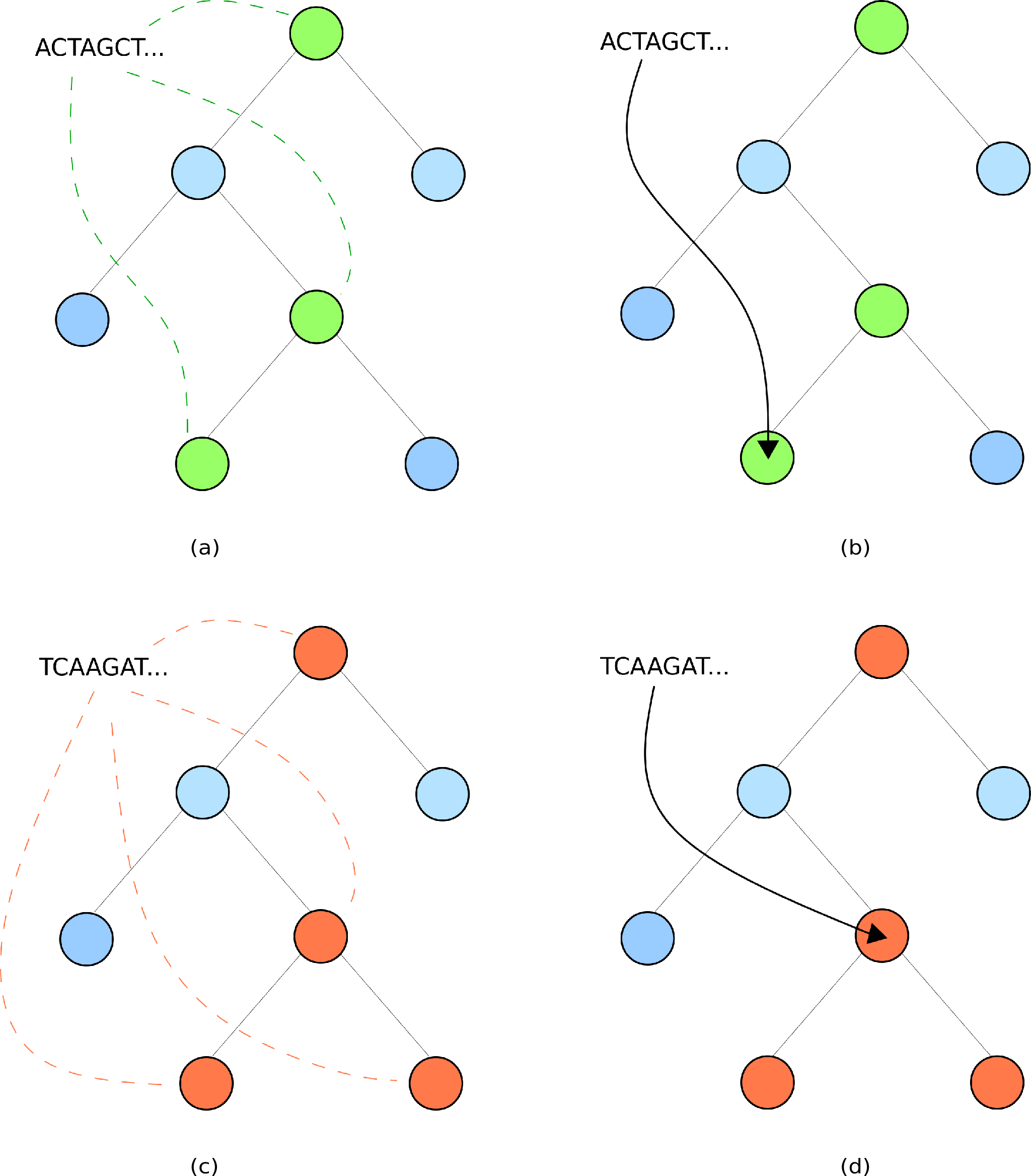
Consider some metagenomic read. From this read, we can extract the corresponding k-mers.

Note

The k-mers of a string are the set of substrings of length k. For example, the 5-mers of ACGTACG are ACGTA, CGTAC and GTACG.

We can map the k-mers of metagenomic reads using the expam database, where k-mers are mapped to the lowest common ancestor of all reference sequences containing this k-mer.
Due to this mapping, the k-mer distribution of any chunk of sequence from some reference genome should lie along a single lineage in the reference tree.

Note

The k-mer distribution of a sequence corresponds to the set of points in the reference tree that k-mers from the sequence got mapped to.

If the k-mer distribution lies along a single lineage, this corresponds to a confident classification.
- In this case, the read is assigned to the lowest point of the k-mer distribution.
- See Figures (a) and (b) below.
If the k-mers diverge along multiple lineages, there are two possible explanations:
1. the sequence has come from a genome that is not in the reference database,
2. a sequencing error has occurred in the form of a base indel/substitution.
In this case, the read is assigned to the lowest point where the lineages agree.
See Figures (c) and (d) below, and note the pressence of two lineages.

Note

Splits can be induced in a read due to sequencing error, which may make some read of a reference genome appear as though it does not below to the genome, as a small number of k-mers from this read will be impacted by the incorrect base.

To overcome this, expam implements an $\alpha$ parameter, to only consider lineages containing more than $\alpha$% of the k-mer distribution. This should ignore those lineages in the k-mer distribution that contain too few k-mers and are most likely due to sequencing error.

What do I do with splits?

As we mentioned above, splits can occur either as a result of sequencing error, or due to novel sequence.
expam implements two strategies to deal with splits as a result of sequencing error:
- The $\alpha$ parameter ignores lineages in a split distribution with low k-mer representation. (See the note above.)
- There are two cutoff flags that can be supplied, which filter out low abundance clades/taxa from the results. These are outlined in the following note.

Note

Sequencing errors can produce spurious classifications that manifest as low abundance clades/taxa in the summary files. These should be filtered out before interpreting the prevalence of clades and species in your sample.

The --cutoff flag sets a minimum count that any clade/taxa needs to reach before it is included in the classification results. The --cpm flag sets the same cutoff, but as a rate of count required per million reads in the sample, as opposed to a flat cutoff number.

When both are supplied, the highest of either cutoff is taken. By default, expam requires each node to have at least 100 counts per million input reads.

With both these mechanisms in place, we can be more confident that high split counts in a particular region of the phylogeny is suggestive of novel sequence in the biological sample.
The algorithm for classifying splits takes a conservative approach - those that are interested only in a general profile can feel comfortable simply adding classification and split counts together to produce an overall profile.
Splits can also be used as a marker for genome discovery - samples reported with a high split counts are potential targets for culturing novel isolates.

Phylogenetic classification results

Say we have just run a sample sample_one.fq against the database, and the classification results are in a folder ./sample_one.
```
$ expam classify -db my_database -d /path/to/sample_one.fq --out sample_one
```
In ./sample_one, there will be a phy subdirectory containing three files:
- ./sample_one/phy/sample_one.csv - sample summary file.
- ./sample_one/phy/classified.csv - complete classifications.
- ./sample_one/phy/split.csv - split classifications.
- Within ./sample_one/phy, there will be a raw subdirectory containing the output for each read.

Sample summary files

Each input sample file gets a corresponding sample summary file.
Comma-separated file of all results for the sample, both complete and split.
There are seven columns:
1. Node - classification point in tree.
Note

If a node points to some location in the reference tree, it will start with a ‘p’.

This point can be used as input to the programmatic tree interface for further analysis.
1. Percent classified (cumulative) - the percentage of all reads classified at or below this node.
2. Total classified (cumulative) - the raw number of reads classified at or below this node.
3. Total classified (raw) - the total number of reads classified at precisely this point.
4. Percent split (cumulative) - the percentage of all reads classified as a split at or below this point.
5. Total split (cumulative) - the total number of reads classified as a split at or below this point.
6. Total split (raw) - the number of reads classified as a split precisely at this node.

Warning

The first row of this file contols those that are unclassified - neither classified nor split.

Example

=================================== =================================== ============================== ======================= ============================== ========================= ==================
Node                                Cumulative Classified Percentage    Cumulative Classified Count    Raw Classified Count    Cumulative Split Percentage    Cumulative Split Count    Raw Split Count
=================================== =================================== ============================== ======================= ============================== ========================= ==================
unclassified                        0.0%                                0                              0                       0.0%                           0                         0
p1                                  100.0%                              1000                           3                       0.0%                           0                         0
p2                                  99.7%                               997                            232                     0.0%                           0                         0
p5                                  76.5%                               765                            0                       0.0%                           0                         0
GCF_000005845.2_ASM584v2_genomic    76.5%                               765                            765                     0.0%                           0                         0
=================================== =================================== ============================== ======================= ============================== ========================= ==================

Note

By default, only nodes with counts (above the cutoff) will be included in these summaries. To include all nodes, add the --keep-zeros flag at classification.

Classification files - classified.csv

Comma-separated matrix - cells contain number of reads classified to specific node (row) within any given sample (column).
This enables phylogenetic comparison of samples.
These classifications correspond to those reads whose k-mer distribution lies on a single lineage (high quality).

Example

=================================== ========================================
Node                                Sample One
=================================== ========================================
unclassified                        0
p1                                  3
p2                                  232
GCF_000005845.2_ASM584v2_genomic    765
=================================== ========================================

Split classification files - split.csv

Comma-separated matrix with same interpretation as classified.csv, only these results are those classifications whose lineage was split.

Note

The rows and columns of classified.csv and split.csv will always line up with eachother.

This is for convenience - those who simply want an overall phylogenetic profile can add these two matrices together without needing to pre-process and align the corresponding rows and columns.

Raw read output

Contains the read-wise output for each input sample file.
Each file is tab-delimited, with five columns:
1. Classification code - one of C (classified), S (split) or U (unclassified).
2. Read ID - unique identifier for each read, taken from the header line of each sequence.
3. Node - the phylogenetic node where each read is classified.
4. Read length - length of the read string.
5. Classification breakdown - this formatted string is a space-delimited summary of where the kmers of this read belonged to. For instance, the summary p4:5 p8:16 p4:198 means that 5 kmers were assigned to node p4, 16 kmers were then assigned to node p8, and finally another 198 kmers were again assigned to p4. These results are reported in order, reading the sequence from left to right.

Taxonomic results

Provided you have run the download_taxonomy command (see section in Commands documentation), you can convert the above phylogenetic results into the taxonomic setting.
The following two commands accomplish this task equivalently:

$ expam classify -d /path/to/reads --out example --taxonomy

$ expam classify -d /path/to/reads --out example
$ expam to_taxonomy --out example

Where before the results directory contained only a phy subdirectory, expam will now also create a tax folder, which will now be populated with the corresponding taxonomic output.

Taxonomic sample summaries

For each sample input file, expam will translate a corresponding taxonomic sample summary.
These are comma-separated matrices with nine columns:
1. Taxon ID - NCBI taxon id.
2. Percent classified (cumulative) - total percentage of reads in this sample classified at or below this taxon id.
3. Total classified (cumulative) - total number of reads classified at or below this taxon id.
4. Classified (raw) - number of reads classified directly to this taxon id.
5. Percent split (cumulative) - total percentage of reads classified as a split, at or below this taxon id.
6. Total split (cumulative) - total number of reads classified as a split, at or below this taxon id.
7. Split (raw) - number of reads classified as a split directly at this taxon id.
8. Rank - taxonomic rank associated with the taxon id.
9. Scientific name (lineage) - (space-separated) taxonomic lineage associated with this taxon id.

Example

=============== =================================== ============================== ======================= ============================== ========================= ================== =============== =================================================================
Node            Cumulative Classified Percentage    Cumulative Classified Count    Raw Classified Count    Cumulative Split Percentage    Cumulative Split Count    Raw Split Count    Rank            Scientific Name
=============== =================================== ============================== ======================= ============================== ========================= ================== =============== =================================================================
unclassified    0.0%                                0                              0                       0.0%                           0                         0                  0               0
1               100.0%                              1000                           0                       0.0%                           0                         0                  root
131567          100.0%                              1000                           0                       0.0%                           0                         0                  top             cellular organisms
2               100.0%                              1000                           235                     0.0%                           0                         0                  superkingdom    cellular organisms Bacteria
1224            76.5%                               765                            0                       0.0%                           0                         0                  phylum          cellular organisms Bacteria Proteobacteria
1236            76.5%                               765                            0                       0.0%                           0                         0                  class           cellular organisms Bacteria Proteobacteria Gammaproteobacteria
=============== =================================== ============================== ======================= ============================== ========================= ================== =============== =================================================================

Note

expam only supplies taxonomic versions for sample summary files, it does not create any taxonomic version of the classified.csv` or splits.csv as in the phylogenetic case.

Taxonomic raw output

expam also translates raw classification outputs for each read into the taxonomic setting.
This is located in ../run_name/tax/raw, again with one summary file per sample.
There are four tab-delimited columns:
1. Classification Code
2. Read ID - unique identifier for each read, taken from header lines of the sequence.
3. Taxon ID - NCBI taxon id that this read was assigned to.
4. Read length - length of the read string.

Example

C       R4825323246286034638    543     302
C       R4280015672552393909    511145  302
S       R5925738157954038177    511145  302
C       R3237657389899545456    511145  302
C       R6111671585932593081    511145  302
C       R4574482278193488645    511145  302

Note

Note the lack of ‘p’ at the start of values in the third column - these refer to NCBI taxonomic IDs, not points in the reference tree.